Understanding Digital Geoscience: Foundations, Methods and Perspectives

Digital geoscience covers every approach that uses digital technologies, mathematical methods and computing tools to acquire, process, represent, model and interpret information about the Earth. More than a discipline with strict borders, it is a cross-cutting field where several areas converge.

Within this field, computational geoscience focuses on formulating problems and solving them numerically. The two terms are close but not interchangeable: digital geoscience also includes data infrastructures, observation platforms, geographic information systems and the digital sharing of knowledge. Nor was it born with artificial intelligence: mathematical modelling, simulation, geophysical inversion and scientific computing have been its foundations for decades. AI enriches this whole without replacing the disciplines that built it.

Suppose we want to study a buried geological formation. We know neither its geometry, nor its physical properties, nor all its boundaries; we only have partial information: geophysical measurements, geological observations, boreholes, satellite data. The digital approach links these observations to a computable representation of the system, in four steps.

Every study starts with data: geophysical surveys, weather stations, hydrological sensors, boreholes, topographic surveys, satellites. None of it is perfect: instrument noise, environmental conditions, measurement errors, acquisition constraints. An observation is often written as signal plus error, $d_{\text{obs}} = d_{\text{true}} + \varepsilon$. The first challenge is therefore not to accumulate data but to assess its quality, representativeness and relevance: a model built on inadequate data can produce convincing results and wrong interpretations.

Conservation laws, constitutive relations and physical equations underpin the representation. Many geophysical phenomena obey a conservation law of the form

where $u$ is the conserved quantity (mass, charge, energy), $\mathbf F$ its flux and $s$ a source term. In hydrogeology, water flux follows Darcy’s law, $\mathbf q = -K\,\nabla h$, where $h$ is hydraulic head and $K$ hydraulic conductivity. Combined with mass conservation, it gives the groundwater flow equation:

with $S_s$ the specific storage and $W$ recharge or pumping. In electromagnetic geophysics, fields obey Maxwell’s equations; at the low frequencies used in exploration (the quasi-static regime) they reduce to

where $\sigma$ is the electrical conductivity of the subsurface, exactly the property we want to image. But geological systems have irregular geometries, heterogeneous properties and non-linear interactions, so an exact analytical solution is hard, often impossible, to obtain.

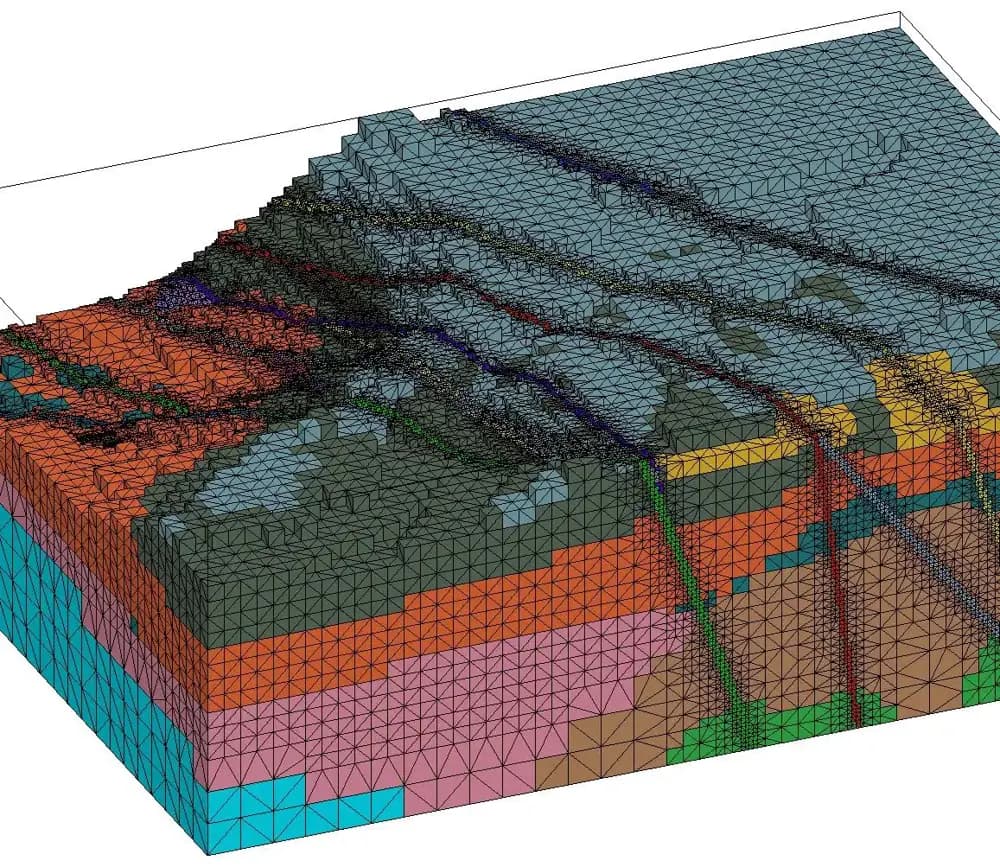
Numerical analysis turns a continuous problem into a discrete representation a computer can solve, using finite differences, finite elements or finite volumes. Instead of treating a watershed as a continuous space, we divide it into cells on which the variables are approximated.

Take equation (2) in one dimension, with constant $K$ and $S_s$. On a grid with spacing $\Delta x$ and time step $\Delta t$, an explicit finite-difference scheme reads

This scheme is stable only if $r \le \tfrac{1}{2}$: a purely numerical constraint dictates the time-step size. Implicit schemes remove the limit at the cost of solving, at every step, a large sparse linear system $A\,\mathbf h = \mathbf b$. This is the core of many hydrological, geophysical, geomechanical and atmospheric simulations.

A simulation is not automatically faithful to the real world, though: its accuracy depends on the model’s assumptions, the discretisation, the parameters and the boundary conditions.

Two questions must be kept apart. Did we solve the chosen equations correctly? That is verification: for example, checking that the error shrinks with mesh size $h$ as $\lVert u_h - u \rVert \le C\,h^{p}$, where $p$ is the order of the method. Do these equations and parameters represent the observed phenomenon well? That is validation, and it requires independent observations.

The rigour of digital geoscience therefore requires confronting models with independent observations, testing their sensitivity to assumptions and quantifying their uncertainties. That critical process is what turns computation into scientific knowledge.

The distinction between forward and inverse problems sits at the heart of many applications. Let $\mathbf m$ be the model (for example resistivity in each cell) and $\mathbf d$ the measured data. Physics links them through a forward operator $F$:

Forward modelling starts from a known model to predict the observations: from a resistivity model, we simulate an electromagnetic response. In the field the problem usually runs the other way: we have measurements and seek the model that explains them. That is the inverse problem.

The difficulty is that several models can produce almost identical responses: with limited, noisy data the solution may be non-unique or unstable (the problem is ill-posed in Hadamard’s sense). We therefore add regularisation, which favours models consistent with prior knowledge, and minimise an objective function:

The first term measures misfit to the data (weighted by their uncertainties through $\mathbf W_d$); the second penalises models that are too rough or too far from a reference model; $\beta$ balances the two. Because $F$ is usually non-linear, we iterate. With $\mathbf J$ the Jacobian (sensitivity) matrix of $F$, a Gauss–Newton update reads:

followed by $\mathbf m_{k+1} = \mathbf m_k + \alpha\,\delta\mathbf m$. The same logic appears in geophysical exploration, seismic imaging, tomography, hydrology and environmental parameter estimation. It shows the power of numerical approaches: using accessible measurements to study properties we cannot observe directly.

Machine learning and deep learning have greatly expanded what we can do with scientific data. A model $f_\theta$ learns its parameters $\theta$ from examples $(\mathbf x_i, y_i)$ by minimising an empirical risk:

Applications abound: classifying satellite images and detecting change in remote sensing; forecasting river flow in hydrology, given suitable data and rigorous validation; supporting interpretation, accelerating computations and estimating parameters in geophysics; analysing factors behind floods and landslides in hazard studies.

Rather than setting physical models against learning algorithms, we can exploit their complementarity: physics brings knowledge of mechanisms, statistics learns complex relationships from data. This convergence takes several forms: a surrogate model that approximates an expensive simulator; a network that builds physical constraints into its training; a hybrid system in which a learned module represents a process the simulator describes poorly.

Physics-informed neural networks (PINNs, Raissi et al., 2019) are one example: they add the residual of the partial differential equation to the data loss. For equation (2), with $h_\theta$ the field predicted by the network:

The second term is evaluated at collocation points $(\mathbf x_j, t_j)$ where no measurement is needed, and $\lambda$ sets the weight of the physics. These approaches are genuinely valuable, but not universally better than classical numerical methods: their efficiency depends on the problem, the computational cost and how hard the optimisation is. Reichstein et al. (2019) highlighted the value of hybrid approaches for connecting deep learning with an understanding of Earth processes.

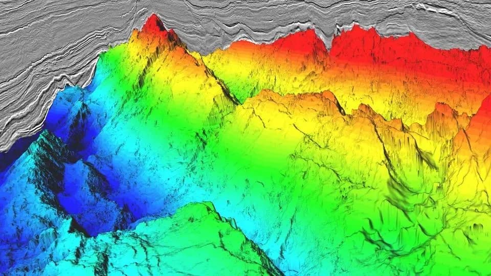
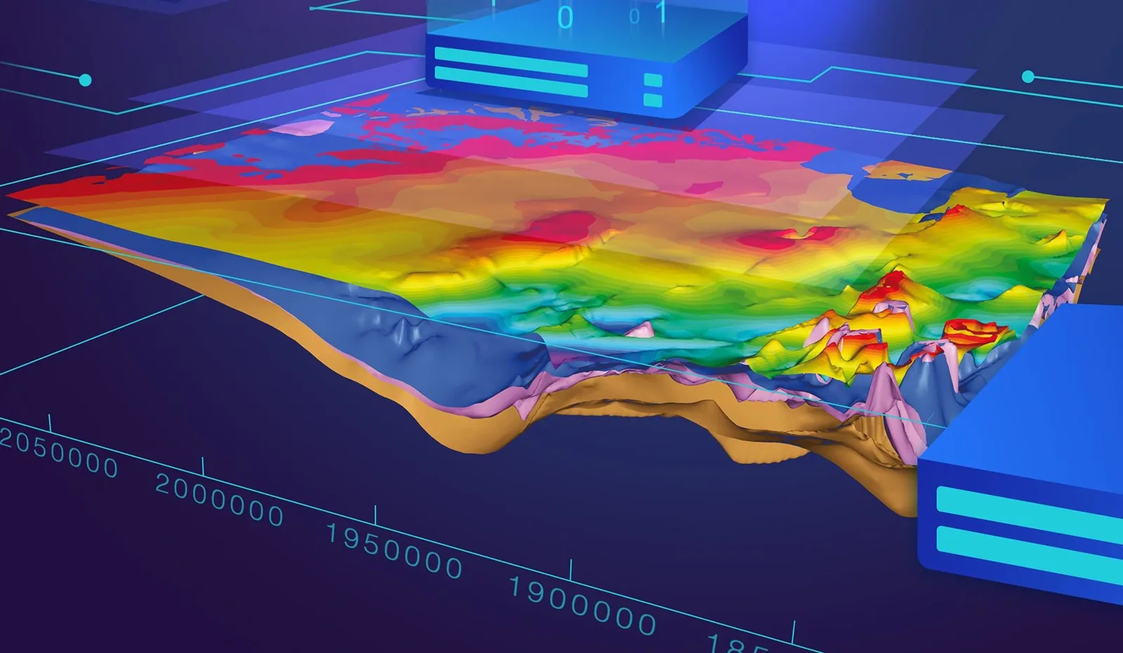
Mineral exploration relies on indirect observations: electrical, electromagnetic, magnetic and seismic methods measure physical properties associated with geological formations. Numerical work comes in to process the signals, solve the inverse problems and produce 2D or 3D images of the subsurface that help pinpoint structures or anomalies of interest.

On their own, these images do not prove mineralisation: their interpretation must be checked against geological data and, where possible, boreholes. Platforms such as pyCSAMT show the value of software development in connecting data processing, modelling and interpretation.

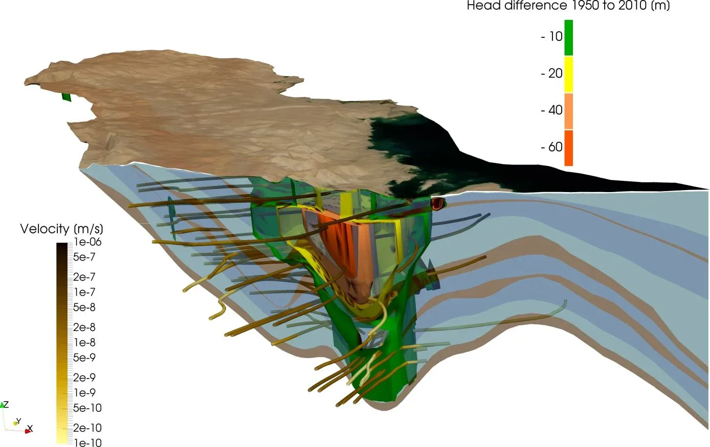
To understand how groundwater moves, hydrogeologists represent aquifers, their hydraulic properties and their exchanges with the environment, and solve equations such as (2) numerically. Tools such as MODFLOW, developed by the USGS, simulate flow and test management scenarios: the effect of pumping, the evolution of water levels, and exchanges between groundwater and surface water.

These models do not replace fieldwork: their reliability depends on the quality of the hydrogeological data and on careful calibration and validation.

Floods show how interdisciplinary the field is: rainfall, digital elevation models, land cover, hydrological measurements and flow equations combine to explore how water might spread under different scenarios. AI can help with forecasting, error correction or faster computation. But uncertainty stays high (future rainfall, initial conditions, hydraulic parameters, data quality): a flood map is the output of a model and a scenario, not a certainty.

Remote sensing, geographic information systems and numerical analysis make it possible to follow deforestation, changing water bodies, land cover and some surface deformation. Time series separate seasonal variation from lasting change; statistical models and machine learning then help interpret them. Digital geoscience is therefore not only about what lies beneath our feet, but also about surface dynamics and their interactions with human activity.

Despite the progress of numerical tools, several difficulties remain.

For uncertainty, the Bayesian framework is especially illuminating: rather than a single model, it describes a distribution of models consistent with the data and prior knowledge,

whose spread measures what the data cannot constrain. Progress therefore does not only mean ever-larger models; it means designing methods that are efficient, transparent and suited to real needs.

In Africa, the stakes around water, mineral exploration, natural hazards, agriculture and the environment are particularly high. Digital geoscience can offer relevant approaches, provided it is built on local scientific realities and data.

The key challenge is scientific and technological autonomy: African universities and laboratories should not be limited to using solutions developed elsewhere, but should help create software, new methods and open datasets. The open-source ecosystem, Python and its libraries in particular, is an opportunity for training and collaboration. Access to technology is not enough, though: mathematical, geological, physical and computing skills remain decisive. In Côte d’Ivoire, applications range from geophysical prospecting to groundwater management, environmental monitoring and flood modelling.

You do not need to master programming, advanced mathematics, physical modelling and AI all at once. The best approach starts from a simple scientific question: a geology student can visualise field data and build a digital map; a hydrology student can analyse rainfall and river-flow series before running a first flow simulation; a geophysics student can explore how subsurface properties relate to measured responses.

Python is often an excellent entry point, with NumPy, SciPy, pandas, Matplotlib and xarray to handle data, compute and visualise. Governing equations, numerical methods, inverse problems and AI come next.

Several trends shape the future: more available Earth observations, high-performance computing, wider use of AI and the growth of open tools. Digital twins, which combine models, observation data and continuous updating, open new possibilities for monitoring some Earth systems; hybrid physics–learning models will remain an active research area. Yet their success will depend less on faster computers or bigger models than on our ability to ask the right questions, develop rigorous methods, share knowledge and train scientists able to look critically at their tools.